Every enterprise search engineer has written the same ugly piece of code at least once. It lives in the indexing pipeline, it is usually called something like CategoryTagger or UrgencyRules, and it is a few hundred lines of keyword lists, regular expressions and if statements that decide which bucket a document goes into before Solr ever sees it. It is brittle, it is never finished, and nobody wants to own it. When language models arrived the obvious move was to replace it with a prompt. That mostly made it slower and less predictable, because a model built to write paragraphs is the wrong tool for answering a multiple-choice question.
Cloudflare’s release of Clef this week, following Typesafe’s Jev a few weeks earlier, puts a name on the tool I actually wanted: a decision model. You hand it some text (or an image), a list of typed questions, and it hands back a probability for every allowed answer. Nothing else. No prose, no JSON to parse, no retry loop when the output is malformed. This post is my attempt to understand how that works mechanically, with some animated mockups, and then to work out what it changes for a Solr index. The short answer is that it changes the index more than the query, which is not where I expected to land.
A decision model answers a form, not a question
The mental model that unlocked it for me: a decision model fills in a form. The caller defines the form. Each field has a type, an instruction, and a closed set of allowed values. The model’s entire output is one probability per allowed value per field. The three field types in the Jev-compatible API map almost exactly onto the field types a search engineer already thinks in:
- Boolean (“noul” in the API). Is this listing a hazardous material? One probability.
- Choice. Which of these categories does it belong to? A probability per category, summing to one.
- Score. An ordered scale. Condition: new, open-box, used, damaged. A probability per step, where being one step off is less wrong than being three steps off.
Here is the same call drawn as motion. I am using a product listing as the running example because that is the shape of most documents I index, and because the questions are the questions a catalog team actually asks.
Two things in that picture matter more than they look. First, the caller owns the schema. Adding a fourth department does not mean retraining anything; it means adding a line to the form. That is the property the old CategoryTagger never had and the reason a general model felt tempting. Second, the probabilities are the product, not a by-product. A generative model can be coaxed into emitting “0.94” as text, but that string is a guess about a number, not a measurement. A decision model’s probability is the thing its loss function was trained on.
Why it is fast: there is no token loop
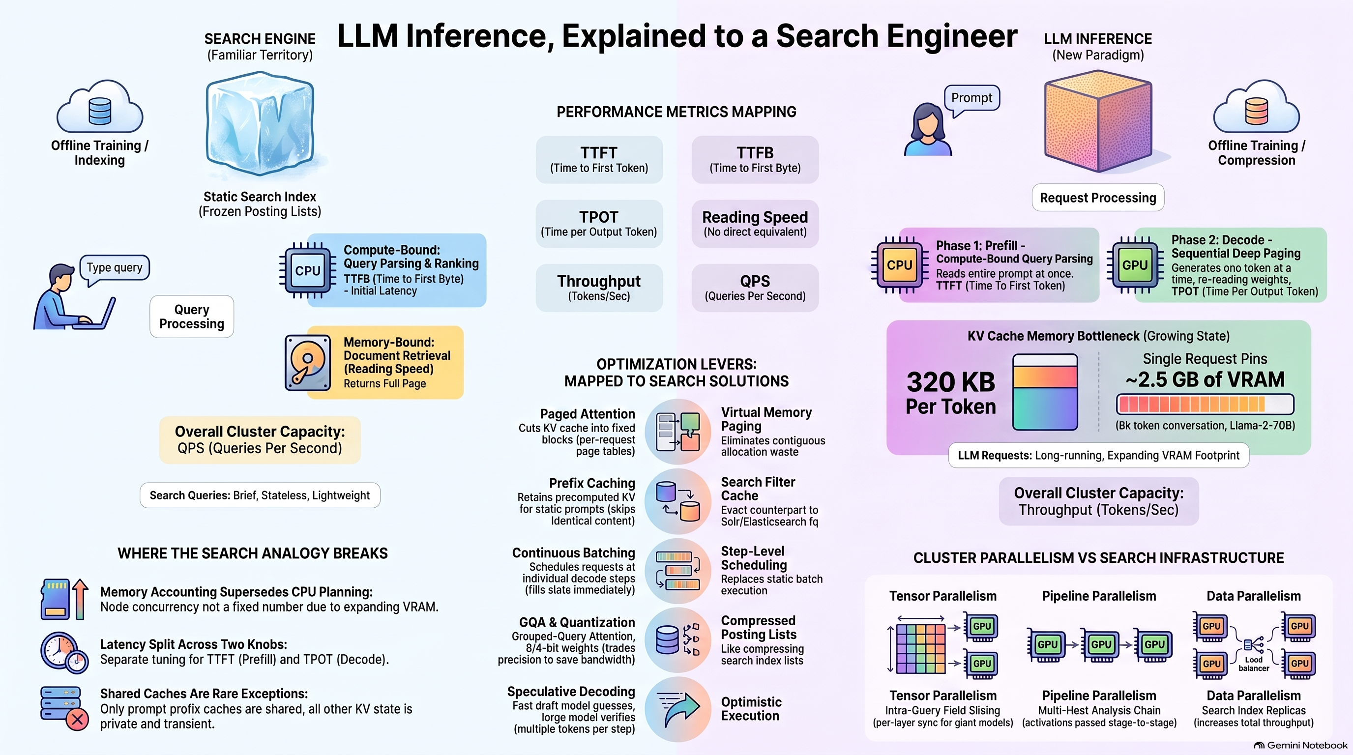
In the last post I described an LLM request as two phases: a parallel, compute-heavy prefill that reads the prompt once, and a strictly sequential decode that produces one token per step. Everything slow about LLM latency lives in decode. Even a short structured answer like {"department":"footwear","condition":"open-box"} is fifteen or twenty tokens, which is fifteen or twenty round trips through the whole model, each one re-reading the weights.
Clef’s central design move is to keep the prefill and delete the decode. The backbone (a frozen Qwen model, 27B parameters for Clef and 9B for Clef-flash) reads the document and the form once. Then a separate scoring head looks at the internal representations that pass produced and assigns a score to every allowed value of every field, all at the same time. Nothing is generated. The answer is non-autoregressive: a single forward pass wide, instead of a chain of passes long.
This is also why I would expect decision models to keep getting cheaper per answer than general models even at equal parameter count. Decode is memory-bandwidth-bound, and the scoring step replaces a long memory-bound chain with one compute-friendly operation. The latency table above is the visible symptom; the hidden one is that a single GPU can serve far more decisions per second than completions.
What the scoring step is actually doing
Cloudflare describes the decision step as a two-stage attention routing process with three ingredients: option-specific evidence routing, joint cross-field attention, and schema-bound scoring with a lexical prior. That sentence is dense, so here is how I have come to picture it, as a search engineer who has built rerankers.
If you have built a cross-encoder reranker, stage one should feel familiar. A cross-encoder scores a (query, document) pair by letting them attend to each other. A decision model is a cross-encoder where the “queries” are the allowed answers and all of them are scored in one shot against one document. The novelty is stage two: in a reranker the candidates never talk to each other, and here they do. That is what lets a form with three interdependent fields come back coherent rather than as three independent guesses.
Calibration is a training target, not a hope
A probability is only useful if 0.9 means “right about nine times in ten”. Most classifiers are overconfident, and most LLM-emitted “confidence scores” are decorative. What I find most interesting in Cloudflare’s write-up is that calibration is a first-class training objective rather than something checked afterwards. Three pieces, in my words:
- Label-smoothed cross-entropy over the valid values. Standard classification loss, but the model is penalised for being certain, which is the first guard against overconfidence.
- Brier loss on top. The Brier score is the squared distance between the predicted probability vector and the truth. Optimising it directly pushes the numbers toward being honest, not just ranked correctly.
- Reinforcement learning for calibrated decisions. A reward that gives partial credit for landing on an adjacent step of an ordered scale, full credit for getting a whole multi-field record exactly right, and a penalty for drifting from the reference model’s behaviour. This is why “used” carried 0.29 in the first figure instead of being crushed to zero: the training signal says near misses on a scale are nearly right.
Only the scoring head and a set of rank-256 low-rank adapters are trained. The backbone is frozen. That matters for the fine-tuning story later, because it means adapting the model to your own labels is a small-parameter job, not a retrain.
Now the Solr part: enrich the index, not the query
Here is where my expectation was wrong. I assumed the interesting use would be at query time, classifying the user’s intent and steering the request. There is a role for that (next section), but the latency budget is tight and the upside is bounded. The larger win is at index time, where latency barely matters, every document is visited anyway, and a well-typed form produces exactly the kind of structured field a Solr schema loves.
The three decision-model field types map onto Solr field types with almost no imagination required:
| Form field | Solr fields it becomes | What it unlocks |
|---|---|---|
| Boolean “hazardous material?” | hazmat_b (boolean) plus hazmat_p (pfloat, the probability) | A hard fq=hazmat_b:false for the storefront; the probability kept so the threshold can move without reindexing the decision. |
| Choice “which department?” | dept_s (string, the argmax) plus dept_p (pfloat) and optionally dept_alt_ss (the runners-up above some floor) | Facets and filters that work for documents the merchant never categorised. The runners-up field lets a listing surface under two departments when the model genuinely cannot tell. |
| Score “condition?” | condition_i (pint, the step index) plus condition_p | Range filters (condition_i:[0 TO 1] for “new or open-box”), sorting, and a boost function that prefers better condition. |
| Any | decision_v (string, model + schema version) | Know which documents were tagged by which model, so a re-tag after fine-tuning can be partial. |
The important design rule is in the second column: store the probability next to the label. The label is for facets and filters. The probability is for everything that needs a knob: a confidence floor on facet counts so that a 0.41 “equipment” guess does not pollute the sidebar, a boost function that trusts strong tags more than weak ones, and a review queue that pulls every document whose top probability fell under 0.6. None of that is possible if you only keep the argmax, and all of it is cheap if you keep one extra float.
Three practical notes from having built pipelines like this with weaker classifiers:
- Do it outside the Solr JVM. A custom
UpdateRequestProcessorthat calls an HTTP model is tempting and wrong; a slow model stalls the indexing thread pool and backs up commits. Put the decision call in the ingestion service that feeds Solr, batch it, and send finished documents. Solr should only ever see completed forms. - Images are now in scope. Clef has a vision encoder, so the form can include “does the photo show the item in its packaging?” or “is this a lifestyle shot or a product shot?” For a catalog, image-derived facets have always been the ones nobody had the data for. Now they are one more field on the form, filled at index time.
- Chunk long documents, then aggregate. A 64k-token context is generous, but a manual or a contract still needs splitting. Run the form per chunk and keep the max probability per value, or better, run a second form over the per-chunk answers. Store which chunk won, because that is what the reviewer will want to see.
Richer output: let the probabilities shape the ranking
Once the fields exist, “richer output” stops being a slogan and becomes a few request parameters. A worked request for the catalog example, written out so the roles are visible:
q        = trail running shoes gore-tex
defType  = edismax
qf       = title^3 description
fq       = hazmat_b:false                      # hard rule from a boolean field
fq       = {!tag=dept}dept_s:footwear         # tagged so the facet stays multi-select
json.facet = {
  dept: { type: terms, field: dept_s,
          domain: { excludeTags: dept,          # multi-select, as usual
                    filter: "dept_p:[0.8 TO *]" } }   # count only confident tags
}
boost    = product(dept_p, recip(condition_i,1,2,2))  # trust strong tags, prefer better condition
fl       = id,title,dept_s,dept_p,condition_i,condition_p

(# comments are mine, not Solr syntax)
Two things here would have been impossible last year. The dept_p floor on the facet means the sidebar is built from decisions the model was sure about, so it stays clean even though every document was tagged automatically. And the boost function uses the model’s confidence as a multiplier, which is a far better signal than the binary “tagged or not” that a rules engine produces. A document the model placed in footwear at 0.94 ranks above one it placed there at 0.81, and both rank above untagged documents, without anyone writing a rule about shoes.
Returning dept_p and condition_p in the field list is deliberate too. The front end can render “Condition: open-box” with a quiet “likely” when the probability is in the middle, and the merchandising team can sort their review queue by it. The number that made the ranking better is the same number that makes the ranking explainable.
Query time: a fast model inside the budget
Query time is where the latency numbers finally matter. A typical interactive search budget is 200 to 300 ms end to end, with Solr itself taking a good share. Clef at ~200 ms median does not fit on that path. Clef-flash at ~40 ms median does, and that changes what is reasonable to do with the user’s query before it reaches the engine.
Within that budget, the forms I would actually run on a query are short and boring, which is the point: Is this a product search or a help search? (route to a different handler). Does it name a department? (the gated filter above). Is this a navigational query for one SKU? (skip the fancy ranking entirely). Each one is a decision I used to make with a regex, and each one now comes with a number that tells me how much to trust it.
The fine-tuning loop is the relevance loop
Cloudflare is pairing the model with a reinforcement-learning fine-tuning service: capture live requests and responses through a gateway, score them, update the adapters, redeploy. Read as a search engineer, that is the learning-to-rank loop with different nouns. We already log queries, we already collect judgements (clicks, add-to-carts, editorial labels), and we already retrain a ranking model from them on a schedule. The decision model slots into the same loop with a cleaner label format, because the form is the label schema. Every document a merchandiser corrects in the review queue is a training example in exactly the shape the model consumes.
Because only the adapters move, a fine-tuned model for your catalog is a small artefact that can sit next to the generic one. Tag with the generic model on day one, collect corrections for a quarter, fine-tune, then re-tag only the documents whose decision_v is stale. That is a partial reindex, not a full one, which is the kind of operational detail that decides whether a team actually does it.
Where this will disappoint you
Calibration is measured on their distribution, not yours. A model that is honest on support tickets can be confidently wrong on industrial fasteners. Hold out a few hundred labelled documents, bin the predictions by probability, and plot accuracy per bin before you set a single threshold. The fq/bq bands above are placeholders until that plot exists.
A closed set is only as good as its definitions. The “criteria” text for each value is doing real work in the scoring; vague descriptions give vague probabilities. Write them the way you would write a facet label for a customer, then test two phrasings.
The small model is not the big model. Clef-flash loses badly on some published benchmarks that Clef wins (the out-of-scope intent set is the striking one). Use the fast model for the query path and the accurate one for the index; do not assume one fits both.
It does not retrieve. A decision model scores what you show it. It will not find the document, and it will not notice the field you forgot to put on the form. Retrieval is still Solr’s job; this makes the documents Solr retrieves better described.
What I would do this quarter
- Pick the three fields in the schema with the worst coverage (the ones merchants leave blank) and write them as a form: one boolean, one choice, one ordered score.
- Run the form over a sample of 2,000 documents with the hosted or self-hosted model, store label and probability, and plot the calibration curve against existing labels.
- Add the fields to the schema with a probability floor on the facet and a
decision_vfield. Re-index the sample into a test collection and compare facet quality side by side. - Only then put the fast model on the query path, behind the confidence gate, with every decision logged.
- Turn the review queue into the training set, and plan the first fine-tune for when it has a few thousand corrections.
The reason I am optimistic about this class of model is not that it is clever, though it is. It is that it produces the one thing a search index has always wanted from machine learning and rarely got: a typed value, in a field the schema already knows how to use, with a number that says how much to believe it.
What is established and what is my framing
| Claim | Status | Basis |
|---|---|---|
| Clef’s prefill-only pass followed by parallel, non-autoregressive scoring; frozen Qwen backbones (27B / 9B); rank-256 adapters; label-smoothed cross-entropy + Brier loss; RL with partial credit for adjacent ordinal values | Reported by Cloudflare | Introducing Clef, Cloudflare blog, 1 Oct 2026. |
| Latency figures (Clef 209 ms, Clef-flash 39 ms, Jev 524 ms median across 43 benchmarks); 64k context; vision encoder; Apache 2.0 weights on Hugging Face | Reported by Cloudflare | Same post. Their hardware, their harness; expect different absolute numbers on your own. |
| The boolean / choice / score field types and the request shape | Established | Jev-compatible API as shown in the post; Typesafe’s Jev introduced the format. |
| Decode is memory-bandwidth-bound and sequential; removing it is the latency win | Established | Standard transformer inference analysis; see my previous post and the PagedAttention paper. |
| Brier score as a calibration measure; label smoothing as an overconfidence guard | Established | Brier (1950); Szegedy et al., 2016 on label smoothing; Guo et al., 2017 on calibration of modern networks. |
| The three-stage picture of the scoring head, and the “lexical prior seeds the option query” reading | My interpretation | Cloudflare’s description is one paragraph; the figure is how I understand it, not a diagram they published. |
| Field mappings, the probability-next-to-label rule, the facet floor, the boost function, the fq/bq/log confidence bands and the 0.5 / 0.85 thresholds | My framing | Design proposals from building Solr enrichment pipelines. The thresholds are placeholders to be replaced by a calibration plot on your data. |
| Probabilities in the figures (0.94, 0.66, 0.97, 0.91) and the ~40 / ~90 / 250 ms budget | Illustrative | Invented to make the mechanics visible. Not measurements. |
This is a week-one read of a model released today. The architecture notes come from a single vendor post, and I have not yet run the weights against a real catalog. Everything in the Solr sections is a plan I intend to test, written down before the testing so that I can be honest later about what held up.