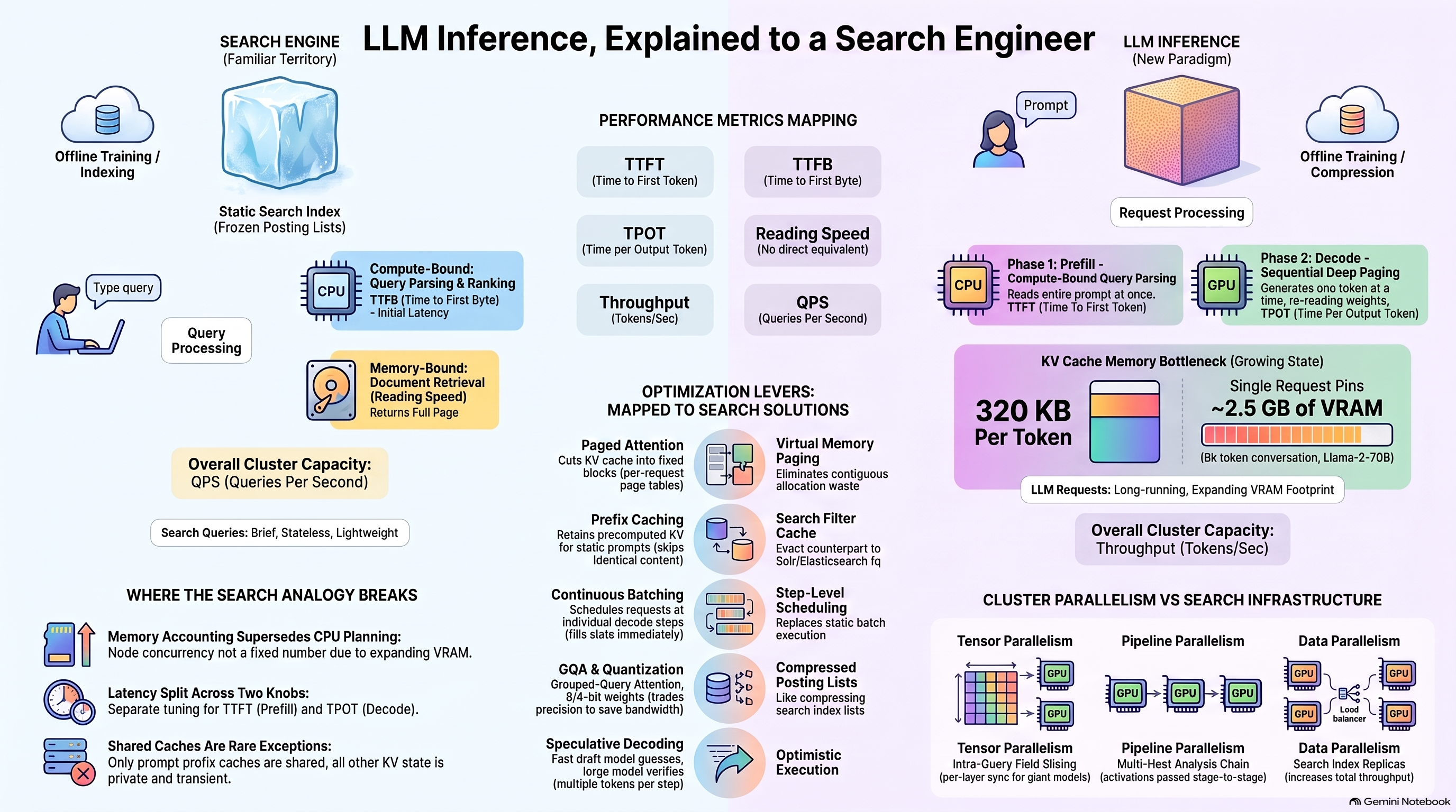
LLM Inference, Explained to a Search Engineer
For most of my career the interesting part of a search engine has been the few hundred milliseconds between a query arriving and a ranked page leaving. Indexing is a batch job you schedule and forget. Query time is where the latency budget, the hardware bill, and the angry tickets all live.
LLM serving has exactly the same shape. Training is the batch job. Inference is query time. And once I started reading inference engineering through that lens, the whole vocabulary — prefill, KV cache, continuous batching, paged attention — stopped looking like new ideas and started looking like old search problems wearing new names. Here is the mapping I now use, plus the places where it breaks.
Training is indexing. The weights are the index.
A search index is a frozen, compressed summary of a corpus, built offline so that queries can be answered without re-reading the documents. Model weights are the same thing one level up: a frozen, compressed summary of a corpus, built offline so that prompts can be answered without re-reading the training data.
That framing settles a question people argue about. “Does the model know X?” is the same kind of question as “is X in the index?” The answer is fixed at build time. Everything that happens afterwards — the request, the scheduling, the caching, the hardware — is inference, and none of it changes what the model knows. It only changes how fast and how cheaply you can ask.
One request, two very different phases
The first thing that surprised me is that a single LLM request is not one workload. It is two, with opposite performance characteristics, glued together.
Prefill reads the whole prompt at once. Every token in the prompt is pushed through every layer of the model in parallel, and for each token the model computes three vectors — a query, a key, and a value — at every layer. This is a big, dense matrix job. The GPU is doing arithmetic flat out. It is compute-bound.
Decode then produces the answer one token at a time. Each new token has to look back at the keys and values of every token that came before it, pick the next word, and append its own key and value to the pile. Each step is small, but the step has to stream the model’s weights through the GPU again from memory. Decode is memory-bandwidth-bound, and it is strictly sequential. You cannot produce token 40 before token 39.
The search analogy I keep coming back to: prefill is parsing and scoring the query against the posting lists, which you can spread across cores and shards. Decode is deep paging with a cursor — page 40 cannot be fetched until page 39 has told you where it ended. The first one scales out. The second one does not, no matter how many GPUs you throw at it.
The KV cache is per-request state, and it grows
Why does decode need all those keys and values from earlier tokens? Because attention is literally “look at every previous token and decide how much it matters.” Without a cache, producing token 500 would mean recomputing the keys and values of tokens 1 through 499 from scratch — quadratic work for a linear answer. So the engine keeps them in GPU memory. That store is the KV cache.
Two properties of the KV cache explain most of inference engineering:
- It is per request. Unlike a search engine’s filter cache, which is shared across every query that uses the same filter, the KV cache belongs to one conversation. Ten concurrent chats mean ten caches.
- It grows with every token, prompt and answer alike. A long system prompt, a pasted document, a long reply: each one claims more GPU memory and holds it until the request finishes.
How much memory? Per token, it is two vectors (key and value), times the number of layers, times the number of KV heads, times the head dimension, times the bytes per number. For a model shaped like Llama-2-70B — 80 layers, 8 KV heads, head dimension 128, 16-bit weights — that works out to about 320 KB per token.
KV bytes per token = 2 × layers × kv_heads × head_dim × bytes_per_value
                   = 2 × 80 × 8 × 128 × 2
                   = 327,680 bytes  ≈ 320 KB

An 8,000-token conversation therefore pins ≈ 2.5 GB of GPU memory,
for one user, before a single new token is produced.
That is the number that reframes everything. GPU memory is the scarce resource, the model weights already take most of it, and what is left over is divided among live conversations. Concurrency on a GPU is not limited by compute. It is limited by how many KV caches fit next to the weights. Every optimisation in the next section is, at bottom, an attack on that constraint.
The front door and the engine room
Anyone who has run Solr or Elasticsearch behind an API will recognise the two-tier layout.
The inference gateway is the front door: authentication, rate limits, per-tenant token budgets, and routing to a pool of GPU workers. It never touches a model. It is the same component as the API gateway in front of a search cluster, and it fails in the same ways — the budget it enforces has to be in the unit that costs you money, which here is tokens, not requests.
The inference engine is the engine room on each worker. It admits requests, batches them, runs prefill, runs decode, owns the KV cache, and streams tokens back. vLLM, TensorRT-LLM, SGLang and friends live here. If the gateway is your load balancer, the engine is the request handler plus the thread pool plus the cache manager, fused into one scheduler because they all contend for the same GPU memory.
Three numbers, and the tension between them
| Metric | What it measures | Which phase drives it | Search-engineer translation |
|---|---|---|---|
| TTFT time to first token | Delay from sending the request until the first token appears | Prefill (plus queueing) | Time to first byte. The “did it hear me?” number. |
| TPOT time per output token | Average gap between tokens once streaming starts | Decode | There is no equivalent; search returns the page in one go. This is the reading-speed number. |
| Throughput tokens per second | Total tokens the system produces across all live requests | Batching efficiency | QPS. The capacity-planning number. |
The tension is the same one every search team already manages between p95 latency and queries per second. Batching more requests together raises throughput, because the expensive weight read is amortised across more tokens, but it stretches each individual request’s TPOT. Serving one request at a time gives the best latency and wastes most of the GPU. The scheduler’s job is to pick a point on that curve, and the right point depends on whether you are serving a chat window or a nightly batch job.
Everything above rolls up into one number the business sees: what it costs to produce a token. It is the same arithmetic as cost per query — hardware-hours divided by useful output. Every lever below either makes each token cheaper or lets the same hardware produce more of them. None of them make the model smarter.
The levers, grouped by what they attack
The inference literature is a long list of named techniques. They are much easier to hold in your head if you sort them by the bottleneck each one is aimed at.
1. Make the KV cache smaller
Grouped-query and multi-query attention (GQA / MQA). In the original transformer every query head has its own key and value heads. GQA lets several query heads share one KV pair; MQA takes it to the limit and gives the whole layer one. The model’s ability to attend barely changes, but the cache shrinks by the sharing factor. This is why that 70B example above has 8 KV heads rather than 64. It is a decision made at training time that pays off at inference time, like choosing docValues over stored fields: you pick the on-disk layout for the query pattern you expect.
Quantization. Store the weights, and sometimes the cache, in fewer bits — 8 or 4 instead of 16. The model gets smaller in memory and, because decode is bandwidth-bound, faster too. The cost is a small, usually acceptable, loss of precision. Search people have been doing this for years under the name “compressed posting lists”: trade a few bits for a lot of bandwidth.
2. Stop wasting the memory you have
Paged attention. Early engines reserved one contiguous slab of GPU memory per request, sized for the longest answer the request might produce. Most answers are shorter, so most of the slab sat empty, and fragmentation between slabs wasted the rest. Paged attention borrows the operating system’s answer: cut the cache into fixed-size blocks, hand them out on demand, and keep a page table per request. Memory that a finished request frees is immediately usable by a new one.
If you have ever watched Lucene’s off-heap segment memory fragment under a churn of merges, this is the exact same disease with the exact same cure.
3. Do not compute the same thing twice
Prefix caching. In a real application nearly every request starts the same way: the same system prompt, the same instructions, the same tool definitions, and only then the user’s actual message. Prefill recomputes keys and values for that shared prefix on every call, which is pure waste. Prefix caching keeps the KV blocks for the shared prefix resident and lets new requests attach to them, so prefill only has to process the part that is actually new.
This is the one technique with an exact search counterpart: it is the filter cache. A constant fq is computed once and reused by every query that carries it, and the win is proportional to how often the same filter recurs. Same here — the win is proportional to how long and how stable your shared prefix is, which is why putting the volatile part of a prompt at the end is not a style preference but a cost decision.
4. Keep the GPU busy
Continuous batching. The naive way to batch is to collect N requests, run them together, and release the batch when the last one finishes. Because answers have wildly different lengths, that means the GPU spends most of each batch generating for one straggler while the other slots sit idle. Continuous batching schedules at the granularity of a single decode step instead: the moment one request emits its final token, a waiting request takes its slot on the very next step.
Speculative decoding. Decode is sequential, but verifying is not. A small, fast draft model guesses the next several tokens; the big model then checks all of them in one parallel pass and keeps the prefix that matches what it would have said. When the draft is right, you get several tokens for the price of one big-model step. When it is wrong, you lose a little work and fall back. It is optimistic concurrency applied to text — and it works because most of the tokens in any answer are easy.
5. Spread the model across machines
When a model does not fit on one GPU, or one GPU cannot serve the load, there are three ways to split it, and they map almost exactly onto sharding and replication.
- Tensor parallelism slices every individual matrix across GPUs, so all of them work on every layer together. It needs a very fast interconnect because the GPUs synchronise on every layer. It is the only way to run a model that is bigger than one GPU’s memory with low latency.
- Pipeline parallelism gives each GPU a contiguous run of layers and passes the activations down the line. Less chatty, but a single request only ever uses one stage at a time, so you need enough concurrent requests to keep every stage busy.
- Data parallelism is replication. Each GPU holds the entire model and the gateway spreads requests across them. It does nothing for a model that does not fit, and everything for one that does.
6. Do not use the big model unless you have to
Model routing and cascading. Put a router in front of several models and send each request to the cheapest one that can handle it: a small model for easy, well-trodden prompts, a large one for the hard tail, a reasoning model when the task demands it. A cascade is the same idea in series — try cheap first, escalate only on low confidence.
This is query routing, and the lesson from search carries over intact: the router is only as good as its ability to judge difficulty before doing the work. Get it wrong one way and you pay for the large model on trivial requests; get it wrong the other way and users get a cheap, wrong answer with great latency. The honest routers measure their own misroutes.
Where the search analogy breaks
Requests are stateful and they grow. A search query holds almost no memory for almost no time. An LLM request holds a KV cache that grows for the entire life of the response. “How many concurrent users can this node take?” has no fixed answer; it depends on how long they talk.
Latency is paid twice. Search has one latency. Inference has a first-token latency and then a sustained per-token latency, and they are tuned by different knobs. A system can have excellent TTFT and unusable TPOT, or the reverse.
The shared cache is the exception, not the rule. In search, nearly every cache is shared across queries. In inference, only the prefix cache is. Everything else is private to one request and dies with it, which is why memory accounting, not CPU accounting, is the planning discipline.
And the model that does not decode at all
Everything above assumes an autoregressive model: produce a token, append it, repeat. Diffusion models — the image and video generators — work the other way around. They start with the entire output as random noise and refine the whole thing at once, over a few dozen steps, with the prompt’s embedding steering each refinement. There is no token loop and no KV cache growing with the answer. The cost is fixed by the step count and the output size, not by the length of a conversation, which makes a diffusion workload far easier to capacity-plan and far harder to stream. Worth knowing, mainly so that nobody tries to apply continuous batching intuitions to an image service.
What I now ask about any inference stack
- What is the KV cache footprint per token for this model at this precision, and how much GPU memory is left after the weights? That is the real concurrency ceiling.
- Is the engine doing continuous batching with paged memory, or static batching? If static, throughput numbers from a benchmark will not survive real traffic.
- Is prefix caching on, and is our prompt laid out to exploit it? Stable prefix first, volatile content last.
- Are TTFT and TPOT reported separately at p50 and p95? A single “latency” number hides which phase is in trouble.
- Is the token budget enforced at the gateway in tokens, per tenant? Requests are the wrong unit; one pasted PDF costs more than a thousand short questions.
- If there is a router, how does it measure its own misroutes?
None of these questions are new. They are the questions I have asked about every search cluster I have inherited, translated. That is the real conclusion: inference engineering is a systems discipline, and if you have run a retrieval system under load, you already know most of it. You just need the dictionary.
What is established and what is my framing
| Claim | Status | Basis |
|---|---|---|
| Prefill is compute-bound and parallel; decode is memory-bandwidth-bound and sequential | Established | Standard description of transformer inference; see the vLLM / PagedAttention paper and NVIDIA’s inference documentation. |
| KV cache per token = 2 × layers × KV heads × head dim × bytes | Established | Follows from the attention mechanism; the 320 KB figure is computed from Llama-2-70B’s published architecture at FP16. |
| Paged attention and continuous batching, as described | Established | Kwon et al., 2023; continuous batching originates with Orca, OSDI 2022. |
| GQA / MQA reduce cache size by the sharing factor | Established | Ainslie et al., 2023; Shazeer, 2019. |
| Speculative decoding verifies draft tokens in one pass | Established | Leviathan et al., 2023; Chen et al., 2023. |
| The search-engine mappings (filter cache, deep paging, shards and replicas) | My framing | Analogies for intuition, not equivalences. The “where it breaks” section is the honest counterweight. |
| The “8,000-token conversation ≈ 2.5 GB” example | Illustrative | Arithmetic from the formula above; a real engine’s overhead and block rounding will move it. |
Engines move fast. Everything here was true of the mainstream open-source stacks when I wrote it; confirm anything load-bearing against the version you actually run.